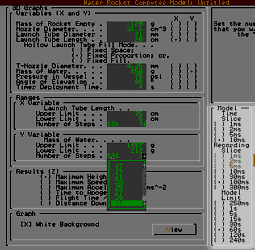
Model time becomes important when there are many, literally hundreds of calculations to perform to fill a graph. You can reduce this time significantly by selecting a longer model Time Slice. Selecting 10ms instead of 1ms will speed things up by an order of magnitude with only a slight increase in error.

10ms and 1ms time slices on small ranges

As the the slice has most effect upon the latter part of flight, errors caused by taking a large time slice manifest themselves most visually on the Flight Time and Distance Downrange graphs. The type of banding is illustrated on the two screen-shots on the left - the banded one at 10ms and the smooth one at 1ms with the ranges quite small.

If you do see errors, they will manifest themselves as bands on the graph. You can make this look worse by selecting a very narrow range for the graph but one thing that you should remember is that the computer model may give peculiar looking results over a range of 0.1grammes of water but in the field, you will find it practical only to measure to the nearest 10 or 20 grammes (or more for wider rockets such as those made from pop bottles).

The recording time slice is irrelevant here as the computer model only monitors the final results from each run.

The model limit is useful if you are looking only at the beginning of the flight, for instance, if you are optimising for a booster where you need the maximum velocity and it is going to happen in the first second of flight. In this case, you can set the Model limit to 1s and the calculation process will be shortened even further.

Finally, for presentations, projects, school/college/university work and so on, where a neat graph is required, remember to make the Model Time Slice 1ms for your presentation plots to give a smooth result as the end result is worth it once you have worked out the limits for each axis of the graph.

Copyright ©2000 Paul Grosse. All Rights Reserved