 Once
you have pressed or clicked on
[View], you are presented with a
screen that looks like the one on the
right. Once
you have pressed or clicked on
[View], you are presented with a
screen that looks like the one on the
right.Normally, when the mouse is
over the grid area, it looks like
this  and when it is over other
areas it looks like this and when it is over other
areas it looks like this  . .
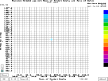
There are a number of things that
you can do with the 3D Optimisation
graphs depending upon what you want.
|
 |
You can
click the mouse on any uncalculated
point to calculate it - during the
calculation, the cursor looks like
this  . . To find out where
the optimum result lies for the two
variables that you have chosen, you
can either fill in the entire grid or
search for the maximum. You can do
these by hand or you can get the
program to do them for you using Fill
and Search
respectively.
|
|
 Pressing Pressing  or clicking on Fill
will fill up the entire grid with
calculated points. This may take some
time depending upon the speed of the
computer running the program, the
number of points and the time slice
that you have selected for the
calculations. or clicking on Fill
will fill up the entire grid with
calculated points. This may take some
time depending upon the speed of the
computer running the program, the
number of points and the time slice
that you have selected for the
calculations.The Fill
function picks grid points at random
so that if you have selected
meaningless grid limits, you will be
able to see that there is going to be
a lack of any useful points early on,
instead of having to wait for the
entire grid to print.
You can terminate the Fill
operation by pressing any key.
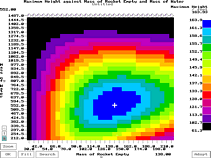
When the screen is full, it should
look something like the screen shot
on the right. As the points are
calculated, the program works out the
range and puts the values for each
colour on the right, effectively
creating a z axis.
As you move the mouse around the
grid, you will see the mouse's x and
y axis values appearing in the bottom
right and top left respectively. You
will also see the z axis value
appearing in the top right. If the
values for a particular point have
caused an error, the appropriate
error message appears instead of the
value.
See  and and  below for another Fill
function. below for another Fill
function.
|
|
 Pressing Pressing  or clicking on Search
will locate the maximum on the grid
much faster. In addition, the speed
is not proportional to the product of
the number of points on the axes but
proportional to their sum thus making
this method faster still. or clicking on Search
will locate the maximum on the grid
much faster. In addition, the speed
is not proportional to the product of
the number of points on the axes but
proportional to their sum thus making
this method faster still. On
selecting Search,
the z axis range is squashed to the
top (see below) so that the top of
the range uses most of the colours,
the mouse cursor changes to this  and you start the search
by clicking somewhere on the grid.
The search function works by
selecting a random direction and a
random rotation (clockwise or
anticlockwise) and then calculates
the point where the mouse was
clicked. It then travels in the
chosen direction, calculating as it
goes, until it comes across a result
that is less than the highest that it
has found so far. It then changes
direction, according to the rotation
that it chose at the beginning, and
calculates that, repeating the search
process until it finds an isolated
maximum. It then produces the eight
pointed star pattern in the screen
shot on the right just in case there
is a lot of granularity in the graph
- it being fairly probable that any
new maximum will be picked up by this
process. and you start the search
by clicking somewhere on the grid.
The search function works by
selecting a random direction and a
random rotation (clockwise or
anticlockwise) and then calculates
the point where the mouse was
clicked. It then travels in the
chosen direction, calculating as it
goes, until it comes across a result
that is less than the highest that it
has found so far. It then changes
direction, according to the rotation
that it chose at the beginning, and
calculates that, repeating the search
process until it finds an isolated
maximum. It then produces the eight
pointed star pattern in the screen
shot on the right just in case there
is a lot of granularity in the graph
- it being fairly probable that any
new maximum will be picked up by this
process.
You can terminate the Search
operation by pressing  . .
This method works fairly well with
roundish shapes but can produce
unreliable results with very thin
diagonal maxima that do not fall at
45 degrees on the grid. To get around
this, simply run the search function
a few times or manually calculate the
points you suspect to be maxima.
|
|
Pressing  or clicking on Zoom
will change the cursor to or clicking on Zoom
will change the cursor to  and you can then select
the lower left corner of the area
that you want to zoom in on. The
program will highlight the grid point
that you click on and you can then
click on the upper right grid point.
Once you have done this, the new
points will be inserted into the
upper and lower limits on the form
and the new graph grid will be
plotted. and you can then select
the lower left corner of the area
that you want to zoom in on. The
program will highlight the grid point
that you click on and you can then
click on the upper right grid point.
Once you have done this, the new
points will be inserted into the
upper and lower limits on the form
and the new graph grid will be
plotted.You can terminate the Zoom
operation by pressing .
|
|
Pressing  or clicking on Adopt
changes the cursor to or clicking on Adopt
changes the cursor to  and you can now select a
point on the grid. The x and y values
of this point will be inserted into
the Input Parameters
form and then copied onto the input
ranges form of the 3D Optimisations
ranges thus providing new ranges. The
Adopt procedure
speeds up considerably the process of
inserting optimised values into the
input parameters sheet and if you
have three parameters to optimise,
you can Search, Adopt, select new
parameter pair, Search, Adopt . . .
and so on until you have the best
starting values for your real rocket.
See Calculations
for some examples of this in action. and you can now select a
point on the grid. The x and y values
of this point will be inserted into
the Input Parameters
form and then copied onto the input
ranges form of the 3D Optimisations
ranges thus providing new ranges. The
Adopt procedure
speeds up considerably the process of
inserting optimised values into the
input parameters sheet and if you
have three parameters to optimise,
you can Search, Adopt, select new
parameter pair, Search, Adopt . . .
and so on until you have the best
starting values for your real rocket.
See Calculations
for some examples of this in action.You
can terminate the Adopt
operation by pressing .
|
|
Pressing  will change the
background from black to white or
back again. It also updates the
checkbox in the Graph
part of the 3D Optimisations page.
Changing the background will not
change the colour scheme that you
have selected although it will redraw
the screen. If you have done
something that has made the system
draw on the screen, such as swapping
to another program and back on some
versions of Windows 95, you can use to redraw if you want. will change the
background from black to white or
back again. It also updates the
checkbox in the Graph
part of the 3D Optimisations page.
Changing the background will not
change the colour scheme that you
have selected although it will redraw
the screen. If you have done
something that has made the system
draw on the screen, such as swapping
to another program and back on some
versions of Windows 95, you can use to redraw if you want.
|
|
Pressing the
number keys will change the type of
graph selected in the order that they
appear on the Results part of the
optimisations page. They are as
follows:
|
| |
| |
 |
|
Maximum
Height; |
| |
 |
|
Maximum
Speed; |
| |
 |
|
Maximum
Acceleration; |
| |
 |
|
Time
to Apogee; |
| |
 |
|
Flight
Time; and, |
| |
 |
|
Distance
Downrange. |
|
| |
In this
way, you can look at the different
graphs with their different outputs
without having to recalculate them
each time.
|
|
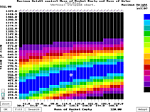 Pressing Pressing  or clicking on the
vertical lined box (on the left) will
split the screen into vertical lines,
each with their own maximum and
minimum. This is what has been done
with the screen shot on the right. or clicking on the
vertical lined box (on the left) will
split the screen into vertical lines,
each with their own maximum and
minimum. This is what has been done
with the screen shot on the right.The
three boxes on the left show the
current status of the screen - on the
right, it is divided into vertical
slices.
If you have the screen sliced like
this and press or Fill,
the cursor changes to  to signify that you can
choose which vertical slice to fill. Fill
works as it does normally with any
key cancelling the process. to signify that you can
choose which vertical slice to fill. Fill
works as it does normally with any
key cancelling the process.
This type of plot is used to find
the best height, flight time and so
on of one variable against another.
In the example on the right, you can
see the best amount of water for any
particular rocket weight. Note that
this is for the specific pressure,
nozzle diameter, coefficient of drag
and so on that was used to obtain the
graph. This type of graph (say for
another example, launch angle for a
given rocket weight giving maximum
downrange distance) can be useful for
taking into the field where you may
not be able to use a computer.
|
|
Pressing or clicking on the
horizontally lined box will divide up
the plot into horizontal slices.
Again, if you have the screen sliced
like this and press or Fill,
the cursor changes to to signify that you can
choose which horizontal slice to
fill. Fill works as
it does normally with any key
cancelling the process.
|
|
Pressing  or clicking on the box
with the square in it will return the
plot to its normal state. or clicking on the box
with the square in it will return the
plot to its normal state.
|
|
Clicking on the
colour scale on the right, or
dragging the mouse up or down it will
squash up the top or bottom of the
scale by varying degrees. This is
done automatically when you go into
Search mode but you can do this for
yourself, selecting the best looking
scale distribution for your purposes.
|
Dark colours at
the top for
a white background. |
|
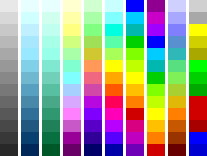
Pressing  will change the colour
set that the plot uses. There are a
number of scales, from monochrome,
through mono-tint to various coloured
scales with some more suited to a
black background and some to a white
background. Pressing repeatedly will simply
cycle through them. will change the colour
set that the plot uses. There are a
number of scales, from monochrome,
through mono-tint to various coloured
scales with some more suited to a
black background and some to a white
background. Pressing repeatedly will simply
cycle through them.
|
|
Pressing or clicking on OK will
exit from the 3D plot.
|
|
Errors are
produced when the model comes across
a situation that is not compatible
with expected flight. If there is not
enough water to get the rocket to the
end of the launch tube, for instance,
this will produce an error which
manifests itself on the plot as a
bubble and when the cursor is over
that point, as an error message
instead of a value. The error
messages are as follows . . .
 |
Error
Message |
|
|
|
Usual
Cause |
|
| |
Low Pressure
|
= |
Not enough
pressure to push out all of
the water. |
|
| |
Low Water
|
= |
All of
the water has been expelled
before the rocket has got to
the end of the launch tube. |
|
| |
Light Rocket
|
= |
Weight of
rocket too low - needs to be
a realistic weight as too low
a weight will generate too
high an acceleration. |
|
| |
Low Capacity
|
= |
Not
enough room for all of the
water you are trying to put
in there. |
|
| |
Small Nozzle
|
= |
The nozzle
diameter is below a lower
limit. |
|
| |
Hole Position
|
= |
Holes
in side of Launch Tube are
too far from the end to be
inside the rocket at the
start of launch. |
|
| |
Small Chute
|
= |
Chute
diameter must be bigger than
that of the rocket. |
|
| |
Vol/Press Err
|
= |
Volume
of liquid too great. |
|
| |
Low Thrust
|
= |
Not enough
thrust to keep the rocket off
the ground until the end of
the water thrust phase. |
|
| |
Low Gas Dnsty
|
= |
Density
of gas is below an arbitrary
limit. |
|
| |
Low Temp
|
= |
Temperature
set below absolute zero. |
|
| |
Short Impulse
|
= |
Air
impulse less than 1ms. |
|
| |
Short L/T
|
= |
Launch tube
less than 1cm long. |
|
| |
L/T Dimensions
|
= |
Launch
tube less than 1mm in
diameter. |
|
| |
Large T-Nozzle
|
= |
T-nozzle
diameter less than 0.01mm or
greater than nozzle diameter. |
|
| |
L/T Thickness
|
= |
Launch
Tube thinckness is greater
than the launch tube radius. |
|
| |
Invalid Angle
|
= |
Angle of
launch less than 5º. |
|
| |
Chute in thrst
|
= |
Chute
opened during water thrust
phase. |
|
| |
Error
|
= |
Anything
else not specified above. |
|
|